


AutoScout24, based in Munich, is one of the largest European online marketplace for buying and selling new and used cars. With its products and services, the car portal is aimed at private consumers, dealers, manufacturers and advertisers. In this post, we use a high-quality car data set from Germany that was automatically scraped from the AutoScout24 and is available on the Kaggle website. This interesting data set comprises more than 45,000 records of cars for sale in Germany registered between 2011 and 2021.
Outline
Let’s first install and import packages we’ll use and set up the working environment:
# Install packages
! uv add lightgbm scikit-optimize category_encoders
import matplotlib.pyplot as plt
import numpy as np
import pandas as pd

from category_encoders import LeaveOneOutEncoder
from lightgbm import LGBMRegressor
import seaborn as sns
from sklearn.compose import ColumnTransformer, TransformedTargetRegressor
from sklearn.metrics import make_scorer, mean_pinball_loss, median_absolute_error
from sklearn.model_selection import cross_val_score, train_test_split
from sklearn.pipeline import Pipeline
from sklearn.preprocessing import OneHotEncoder, PowerTransformer, RobustScaler
from sklearn import set_config
from skopt import gp_minimize, space
from skopt.utils import use_named_args
# Settings
%config InlineBackend.figure_format = 'retina'
sns.set_theme(font_scale=1.5, rc={'lines.linewidth': 2.5})
Quantile Loss Function (aka Pinball Loss Function)
Instead of only reporting a single best estimate, we want to predict an estimate and uncertainty as to our estimate. This is especially challenging when that uncertainty varies with the independent variables. A quantile regression is one method for estimating uncertainty which can be used with our model (gradient boosted decision trees).
A quantile is the value below which a fraction of observations in a group falls.
By minimizing the quantile loss, \(\alpha 100\) of the observations should be smaller than predictions (\(y^{(i)} \lt \hat{y}^{(i)}\)), and \((1-\alpha).100\, \%\) should be bigger (\(y^{(i)} \ge \hat{y}^{(i)}\)).
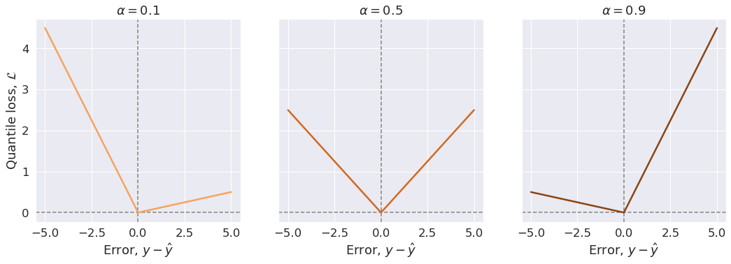
In other words, the model should over-predict \(\alpha.100\,\%\) of the times, and under-predict \((1-\alpha).100\, \%\) of the times. Note that, here the error is defined as \(y - \hat{y}\). As an example, a prediction for quantile \(\alpha=0.9\) should over-predict \(90\%\) of the times.
The quantile loss function is defined as below:
\[\begin{equation} \mathcal{L}_{\alpha}(y^{(i)}, \hat y^{(i)}) = \begin{cases} \begin{aligned} \alpha\,&(y^{(i)} - \hat y^{(i)}) && \text{if} \, y^{(i)} \ge \hat y^{(i)}\quad \text{(i.e., under-predictions)}, \\ (\alpha - 1)\,&(y^{(i)} - \hat y^{(i)}) && \text{if} \, y^{(i)} \lt \hat y^{(i)}\quad \text{(i.e., over-predictions)}, \end{aligned} \end{cases} \end{equation}\]For a set of predictions, the total cost is its average. Therefore, the cost function will be:
\[\begin{equation} \mathcal{J} = \frac{1}{m} \Sigma_{i=1}^m \mathcal{L}_{\alpha}(y^{(i)}, \hat y^{(i)}), \end{equation}\]We can see that the quantile loss differs depending on the evaluated quantile value, \(\alpha\). The closer the \(\alpha\) is to 0, the more this loss function penalizes over-predictions (negative errors). As the \(\alpha\) value gets closer to 1, the more this loss function penalizes under-predictions (positive errors). Figure below illustrates this.
def quantile_loss(y_true, y_pred, alpha):
    """
    Quantile loss function.

    Parameters
    ----------
    y_true : ndarray
        True observations (i.e., labels).
    y_pred : ndarray
        Model predictions (same shape as `y_true`).
    alpha : float
        Evaluated quantile values. Should be between 0 and 1.
    """
    errors = y_true - y_pred
    pos = errors >= 0.0
    neg = np.logical_not(pos)
    loss_vals = alpha * (pos * errors) + (alpha - 1) * (neg * errors)
    return loss_vals
For the sake of illustration, we consider one single true value and investigate how the quantile loss function behaves when model predictions are larger than the true value (negative erros) or smaller that that (positive errors) for different quantile values \(\alpha\).
y_true = 5.0
y_pred = np.linspace(0.0, 10, 51)
errors = y_true - y_pred

# Quantile values
alphas = [0.1, 0.5, 0.9]
colors = ['sandybrown', 'chocolate', 'saddlebrown']

fig, axes = plt.subplots(1, 3, sharey=True, figsize=(15, 5))
fig.tight_layout(w_pad=1)
axline_kw = dict(ls='--', lw=1.5, c='gray')

for alpha, color, ax in zip(alphas, colors, axes):
    ax.axvline(0.0, **axline_kw)
    ax.axhline(0.0, **axline_kw)

    loss_vals = quantile_loss(y_true, y_pred, alpha)
    ax.plot(errors, loss_vals, color)
    ax.set(title=fr'$\alpha={alpha}$', xlabel=r'Error, $y - \hat{y}$')

axes[0].set_ylabel(r'Quantile loss, $\mathcal{L}$');
Data Loading
Let’s load our data set that we have analysed and cleaned previously.
cars = pd.read_csv('../data/autoscout24_germany_dataset_cleaned.csv')
cars.sample(frac=1).head(n=10)
| mileage | make | model | fuel | gear | price | hp | age | |
|---|---|---|---|---|---|---|---|---|
| 3206 | 26566 | Fiat | 500 | Gasoline | Manual | 8240 | 69.0 | 4 |
| 2076 | 92000 | Mitsubishi | Space Star | Gasoline | Manual | 5399 | 71.0 | 6 |
| 8537 | 101709 | smart | forTwo | Gasoline | Automatic | 8490 | 102.0 | 10 |
| 502 | 20302 | Ford | Galaxy | Diesel | Manual | 28711 | 190.0 | 3 |
| 37020 | 79500 | Ford | Edge | Diesel | Automatic | 28740 | 209.0 | 5 |
| 9958 | 38335 | Hyundai | i20 | Gasoline | Manual | 12470 | 84.0 | 4 |
| 3856 | 74860 | Volkswagen | up! | Gasoline | Manual | 5500 | 75.0 | 10 |
| 10262 | 106000 | Ford | Galaxy | Diesel | Automatic | 14000 | 163.0 | 7 |
| 23216 | 29450 | Ford | Focus | Gasoline | Manual | 16450 | 140.0 | 4 |
| 22424 | 50000 | Mercedes-Benz | Sprinter | Diesel | Manual | 17990 | 114.0 | 5 |
Preparatory Feature Selection
We do not utilize 'model' column since it is a subset of 'make' (car brand) feature and each car brand has its own set of model categories, that is not the same for other car brands. It is better to use this column when predicting the sale price of a specific car make, e.g. BMW, is aimed.
cars.drop(columns=['model'], inplace=True)
cars.head()
| mileage | make | fuel | gear | price | hp | age | |
|---|---|---|---|---|---|---|---|
| 0 | 235000 | BMW | Diesel | Manual | 6800 | 116.0 | 11 |
| 1 | 92800 | Volkswagen | Gasoline | Manual | 6877 | 122.0 | 11 |
| 2 | 149300 | SEAT | Gasoline | Manual | 6900 | 160.0 | 11 |
| 3 | 96200 | Renault | Gasoline | Manual | 6950 | 110.0 | 11 |
| 4 | 156000 | Peugeot | Gasoline | Manual | 6950 | 156.0 | 11 |
Data Splitting
We use \(80\%\) of samples in the training set, while the remaining samples (\(20\%\)) will be available in the testing set.
data = cars.drop(columns='price', inplace=False)
target = cars['price']

X_train, X_test, y_train, y_test = \
    train_test_split(data, target, test_size=0.2)
Leave-One-Out Encoding
Our data consists a mixture of numerical and categorical features. More specifically, ('mileage', 'hp', 'age') are the numerical features, and ('make', 'fuel', 'gear') are the categorical features. In orther to be fed into a machine-learning model, categorical features should be represented numerically.
for feature in ('make', 'fuel', 'gear'):
    print(
        f'Feature: {feature} - '
        f'Number of categories: {data[feature].nunique()}')
Feature: make - Number of categories: 72
Feature: fuel - Number of categories: 4
Feature: gear - Number of categories: 3
To encode the features 'fuel' and 'gear', we use the most commonly used method one-hot encoding (sometimes called “dummy encoding”). This algorithm creates a binary variable for each unique value of the categorical variables (for each sample, the new feature is 1 if the sample’s category matches the new feature, otherwise the value is 0). This algorithm adds a new feature for each unique category in 'fuel' and 'gear'.
Since the category 'make' in our data set comes with high cardinality (i.e., it has too many unique categories), using one-hot encoding for this feature will create too many additional feature variables. This could lead to poor model performance - as data dimentionality increases, the model suffers from the curse of dimensionality).
To keep the number of dimensions under control, we use leave-one-out encoding method. It essentially calculates the mean of the target variables over all samples that have the same value for the categorical-feature variable in question. The encoding algorithm is slightly different between training and testing sets:
- For training set, it leaves the sample under consideration out, hence the name Leave One Out. This is done to avoid target leakage. Moreover, it adds random Gaussian noise with zero mean and \(\sigma\) standard deviation into training data in order to decrease overfitting. \(\sigma\) is a hyperparameter that should be tuned.
- For testing set, it does not leave the current sample out - the statistics about target variable for each value of each categorical variable calculated for the training data set is used. It also does not need the randomness factor.
Leave-one-out technique is implemented in the Category Encoders library as a scikit-learn-style transformer:
loo_encoder = LeaveOneOutEncoder(sigma=0.05)
encoded = loo_encoder.fit_transform(X_train['make'], y_train)
encoded.head(n=10)
| make | |
|---|---|
| 38370 | 9573.924156 |
| 13498 | 9029.417690 |
| 27888 | 8792.132242 |
| 12999 | 25944.844420 |
| 7243 | 9101.103968 |
| 2653 | 12284.006678 |
| 7050 | 13583.914503 |
| 31847 | 14364.409615 |
| 1741 | 8766.192993 |
| 36229 | 8188.430674 |
Box-Cox Transformation of Targets
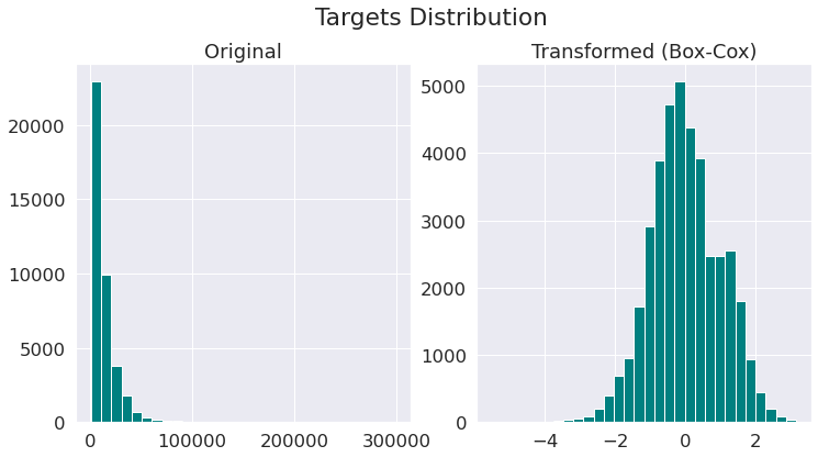
In the previous notebook, where we did the exploratory data analysis, we saw that the distribution of the target variables (prices) in our data set is very skewed to the left. We also saw that the target variables show unequal variability when monitored over different indipendent variables (see cone-shape scatter plots there). This is a sign of heteroscedasticity.
Although, we will use a tree-based learning algorithm that does not make any assumptions on normality of the targets, it would be useful to make targets more Gaussian-like for modeling issues related to heteroscedasticity (non-constant variance).
Here, we use Box-Cox transformation to map targets to as close to a Gaussian distribution as possible in order to stabilise the variance and minimize the skewness. Note that Box-Cox transform can only be applied to strictly positive data (such as income, price etc).
pt = PowerTransformer(method='box-cox')
y_orig = target.values[:, np.newaxis]
y_norm = pt.fit_transform(y_orig)

fig, (ax1, ax2) = plt.subplots(1, 2, figsize=(12, 6))
plt.suptitle('Targets Distribution', y=1)

hist_kw = dict(bins=30, facecolor='teal')

_ = ax1.hist(y_orig, **hist_kw)
ax1.set_title('Original')

_ = ax2.hist(y_norm, **hist_kw)
ax2.set_title('Transformed (Box-Cox)');
Creating Model Pipeline Step by Step
Data-Preprocessing and Transformation
- Robust scaling for numerical features
- One-hot encoding for
'fuel'and'gear' - Leave-one-out encoding for
'make'
def create_preprocessor():
    """
    Data preprocessing and feature transformation pipeline

    Returns
    -------
    out : `sklearn.compose.ColumnTransformer` object
    """
    # Numerical features
    numerical_features = ['mileage', 'hp', 'age']
    numerical_transformer = RobustScaler()

    # Categorical features
    categorical_features_a = ['fuel', 'gear']
    categorical_transformer_a = OneHotEncoder(handle_unknown='ignore')

    categorical_features_b = ['make']
    categorical_transformer_b = Pipeline(
        steps=[
            ('loo_encoder', LeaveOneOutEncoder()),
            ('scaler', RobustScaler())])

    # Preprocessing pipeline
    preprocessor = ColumnTransformer(
        transformers=[
            ('numer', numerical_transformer, numerical_features),
            ('categ_a', categorical_transformer_a, categorical_features_a),
            ('categ_b', categorical_transformer_b, categorical_features_b)])

    return preprocessor
LightGBM Regression Estimator
LightGBM is a gradient boosting tree-based framework developed by Microsoft. Fast training, accuracy, and efficient memory utilisation are its main features. LightGBM uses a leaf-wise tree growth algorithm that tends to converge faster compared to depth-wise growth algorithms. It can be a go-to model for many tabular-data machine-learning problems.
LightGBM has several parameters which control how the decision trees are constructed, including:
num_leaves: maximum number of leaves in one tree. Large values increase accuracy on the training set, but also increase the chance of getting hurt by overfitting.max_depth: limit the maximum depth for tree model. It controls the maximum number of splits in the decision trees.n_estimators: number of boosting iterations (trees to build). The more trees built the more accurate the model can be at the cost of longer training time and higher chance of overfitting.learning_rate: the shrinkage rate used for boosting.
We will use Bayesian optimization to find a good combination of these hyperparameters.
To create our regression estimator:
- We use
LightGBMRegressormodel with quantile loss function to estimate the predictive intervals on our dataset. - As discussed before, we regress on transformed targets (Box-Cox transformation). To do so, we need to wrap LightGBM’s regressor by scikit-learn’s
TransformedTargetRegressor.
def create_quantile_regressor(alpha=0.5):
    """
    LightGBM regressor w/ quantile loss applied on transformed targets.
    In the regression problem, targets (prices) are transformed by using
    Box-Cox power transform method, `PowerTransform(method='box-cox')`.

    Parameters
    ----------
    alpha: float
        The coefficient used in quantile-based loss, should be between 0
        and 1. Default: 0.5 (median).

    Returns
    -------
    Quantile regressor to apply on transformed targets.
    """
    ttq_regressor = TransformedTargetRegressor(
        regressor=LGBMRegressor(objective='quantile', alpha=alpha),
        transformer=PowerTransformer(method='box-cox'))

    return ttq_regressor
Full Training Pipeline
def create_full_pipeline(alpha=0.5):
    """
    Full prediction pipeline.

    Parameters
    ----------
    alpha: float
        The coefficient used in quantile-based loss, should be between 0
        and 1. Default: 0.5 (median).

    Returns
    -------
    Pipeline of data transforms with the final estimator returned as
    `sklearn.pipeline.Pipeline` object.
    """
    preprocessor = create_preprocessor()
    ttq_regressor = create_quantile_regressor(alpha=alpha)
    model = Pipeline(
        steps=[
            ('preprocessor', preprocessor),
            ('ttq_regressor', ttq_regressor)])

    return model
set_config(display='diagram')
create_full_pipeline()
Pipeline(steps=[('preprocessor',
                 ColumnTransformer(transformers=[('numer', RobustScaler(),
                                                  ['mileage', 'hp', 'age']),
                                                 ('categ_a',
                                                  OneHotEncoder(handle_unknown='ignore'),
                                                  ['fuel', 'gear']),
                                                 ('categ_b',
                                                  Pipeline(steps=[('loo_encoder',
                                                                   LeaveOneOutEncoder()),
                                                                  ('scaler',
                                                                   RobustScaler())]),
                                                  ['make'])])),
                ('ttq_regressor',
                 TransformedTargetRegressor(regressor=LGBMRegressor(alpha=0.5,
                                                                    objective='quantile'),
                                            transformer=PowerTransformer(method='box-cox')))])
Please rerun this cell to show the HTML repr or trust the notebook.Pipeline(steps=[('preprocessor',
ColumnTransformer(transformers=[('numer', RobustScaler(),
                                 ['mileage', 'hp', 'age']),
                                ('categ_a',
                                 OneHotEncoder(handle_unknown='ignore'),
                                 ['fuel', 'gear']),
                                ('categ_b',
                                 Pipeline(steps=[('loo_encoder',
                                                  LeaveOneOutEncoder()),
                                                 ('scaler', RobustScaler())]),
['make'])])),
('ttq_regressor',
TransformedTargetRegressor(regressor=LGBMRegressor(alpha=0.5,
                                                   objective='quantile'),
transformer=PowerTransformer(method='box-cox')))])ColumnTransformer(transformers=[('numer', RobustScaler(),
['mileage', 'hp', 'age']),
('categ_a',
OneHotEncoder(handle_unknown='ignore'),
['fuel', 'gear']),
('categ_b',
Pipeline(steps=[('loo_encoder',
LeaveOneOutEncoder()),
('scaler', RobustScaler())]),
['make'])])['mileage', 'hp', 'age']
RobustScaler()
['fuel', 'gear']
OneHotEncoder(handle_unknown='ignore')
['make']
LeaveOneOutEncoder()
RobustScaler()
TransformedTargetRegressor(regressor=LGBMRegressor(alpha=0.5,
objective='quantile'),
transformer=PowerTransformer(method='box-cox'))LGBMRegressor(alpha=0.5, objective='quantile')
PowerTransformer(method='box-cox')
Hyperparameter Tuning with scikit-optimize
Objective
def hyperparameter_tuner(model, X, y, search_space, cvs_params, gp_params):
    """
    Parameters
    ----------
    model : estimator object implementing `fit()` method
        The object to use to fit the data.
    X : array-like of shape (n_samples, n_features)
        The data to fit.
    y : array-like of shape (n_samples,) or (n_samples, n_outputs)
        The target variable to try to predict.
    search_space : list, shape (n_dims,)
        List of hyperparameter search space dimensions.
    cvs_params : dict
        Parameters for Scikit-Learn's `cross_val_score()` method.
    gp_params : dict
        Parameters for Scikit-Optimize's `gp_minimize()` method.

    Returns
    -------
    The Gaussian Processes optimization result with the required
    information, returned as SciPy's `OptimizeResult` object.
    """
    @use_named_args(search_space)
    def objective_func(**params):
        """
        Function to *minimize*. Decorated by the `use_named_args()`, it
        takes named (keyword) arguments and returns the objective value.
        """
        model.set_params(**params)
        scores = cross_val_score(model, X, y, **cvs_params)
        return -1.0 * np.mean(scores)

    # We are now ready for sequential model-based optimization
    optim_result = gp_minimize(objective_func, search_space, **gp_params)
    return optim_result
Optimization
%%time

# Parameters of a Scikit-Learn estimator in a pipeline are accessed
# using the `<estimator>__<parameter>` syntax. Valid parameter keys
# can be listed with model's `get_params()` method.

# Hyperparameters search space
search_space = [
    space.Real(
        0.01, 0.6, prior='log-uniform',
        name='preprocessor__categ_b__loo_encoder__sigma'),
    space.Integer(10, 50, name='ttq_regressor__regressor__num_leaves'),
    space.Integer(2, 30, name='ttq_regressor__regressor__max_depth'),
    space.Real(
        0.01, 0.5, prior='log-uniform',
        name='ttq_regressor__regressor__learning_rate')]

# Parameters that'll be passed to sklearn's `cross_val_score()`
cvs_params = {'cv': 3, 'n_jobs': 4}

# Parameters that'll be passed to skopt's `gp_minimize()`
gp_params = {'n_calls': 50,
             'n_initial_points': 10,
             'acq_func': 'EI',
             'n_jobs': 4,
             'verbose': False}

# Lower, middle and higher quantiles to evaluate: lower/upper bounds + median
quantiles = {'q_lower': 0.025, 'q_middle': 0.5, 'q_upper': 0.975}

# Cache Gaussian Process optimization results
cache_gp_results = dict()

for q_level, alpha in quantiles.items():
    print(f'\nHyperparameter optimization for quantile regressor with '
          f'alpha={alpha:.3f} ..... ', end='')

    # Create model pipeline
    model = create_full_pipeline(alpha=alpha)

    # Cross-validation scoring strategy
    scorer = make_scorer(
        mean_pinball_loss, alpha=alpha, greater_is_better=False)
    cvs_params['scoring'] = scorer

    # Find optimal hyperparameters
    gp_result = hyperparameter_tuner(
        model, X_train, y_train, search_space, cvs_params, gp_params)

    # Cache current results
    cache_gp_results[q_level] = gp_result
    print('Done')

    # Report GP optimization result
    print('Best parameters:')
    for i_param, param_value in enumerate(gp_result.x):
        param_name = search_space[i_param].name.split('__')[-1]
        print(''.rjust(4) + f'{param_name}: {param_value:.6f}')
    print('=' * 40)
Hyperparameter optimization for quantile regressor with alpha=0.025 ..... Done
Best parameters:
    sigma: 0.01
    num_leaves: 20
    max_depth: 6
    learning_rate: 0.320519
========================================

Hyperparameter optimization for quantile regressor with alpha=0.500 ..... Done
Best parameters:
    sigma: 0.01
    num_leaves: 41
    max_depth: 27
    learning_rate: 0.197304
========================================

Hyperparameter optimization for quantile regressor with alpha=0.975 ..... Done
Best parameters:
    sigma: 0.01
    num_leaves: 31
    max_depth: 19
    learning_rate: 0.157132
========================================
CPU times: user 3min 1s, sys: 3.07 s, total: 3min 4s
Wall time: 2min 15s
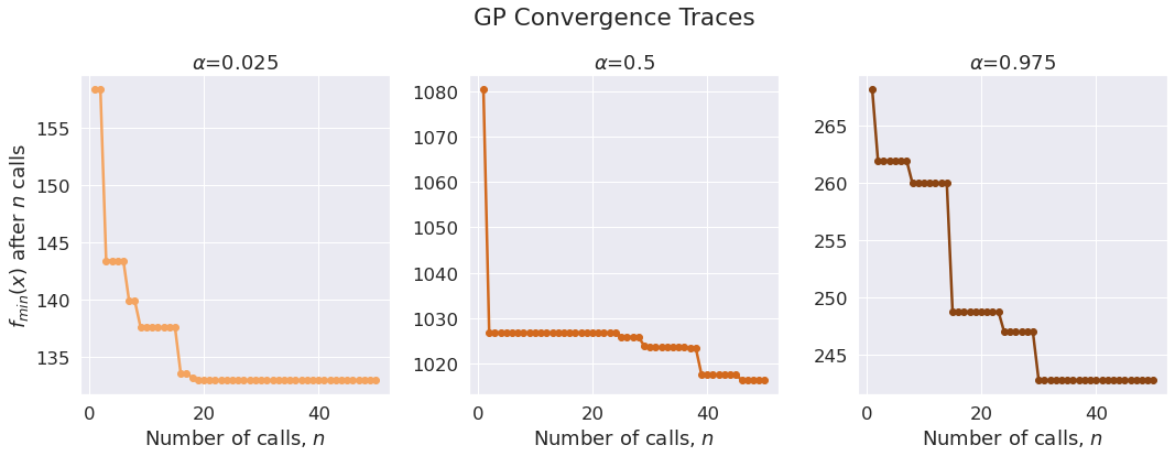
Plotting Convergence Traces
n_models = len(quantiles)
fig, axes = plt.subplots(1, n_models, figsize=(15, 5))
fig.tight_layout(w_pad=1)

colors = ['sandybrown', 'chocolate', 'saddlebrown']

for i, (q_level, gp_result) in enumerate(cache_gp_results.items()):
    call_idx = np.arange(1, gp_result.func_vals.size + 1)
    min_vals = [gp_result.func_vals[:i].min() for i in call_idx]

    ax = axes[i]
    ax.plot(call_idx, min_vals, '-o', color=colors[i])

    alpha = quantiles[q_level]
    ax.set(xlabel=r'Number of calls, $n$', title=fr'$\alpha$={alpha}')

axes[0].set_ylabel(r'$f_{min}(x)$ after $n$ calls')
plt.suptitle('GP Convergence Traces', y=1.1);
Final Estimators: Computing Predictive Intervals
trained_models = dict()

for q_level, alpha in quantiles.items():
    # Create model for this quantile
    model = create_full_pipeline(alpha=alpha)

    # Retrieve best (optimized) parameters for this model
    gp_res = cache_gp_results[q_level]
    n_params = len(search_space)
    best_params = dict(
        (search_space[i].name, gp_res.x[i]) for i in range(n_params))

    # Set the parameters of this model
    model.set_params(**best_params)

    model.fit(X_train, y_train)
    trained_models[q_level] = model
def coverage_percentage(
        y: np.ndarray,
        y_lower: np.ndarray,
        y_upper: np.ndarray) -> float:
    """
    Function to calculate the coverage percentage of the predictive
    interval, i.e. the percentage of observations that fall between the
    lower and upper bounds of the predictions.

    Parameters
    ----------
    y : ndarray of shape (n_samples,)
        Target values.
    y_lower : ndarray of shape (n_samples,)
        Lower predictive intervals.
    y_upper : ndarray of shape (n_samples,)
        Upper predictive intervals.
    """
    return np.mean(np.logical_and(y > y_lower, y < y_upper)) * 100.0
# Compute predictive intervals

y_pred_lower = trained_models['q_lower'].predict(X_test)
y_pred_upper = trained_models['q_upper'].predict(X_test)

ctop = coverage_percentage(y_test, y_pred_lower, np.inf)
cbot = coverage_percentage(y_test, -np.inf, y_pred_upper)
cint = coverage_percentage(y_test, y_pred_lower, y_pred_upper)

print(f'Coverage of top 95%: {ctop:.1f}%',
      f'Coverage of bottom 95%: {cbot:.1f}%',
      f'Coverage of 95% predictive interval: {cint:.1f}%', sep='\n')
Coverage of top 95%: 97.4%
Coverage of bottom 95%: 97.0%
Coverage of 95% predictive interval: 94.4%
y_pred_middle = trained_models['q_middle'].predict(X_test)

print(
    f'Median Absolute Error: ',
    f'\tLower-quantile model: {int(median_absolute_error(y_test, y_pred_lower))}',
    f'\tMiddle-quantile model: {int(median_absolute_error(y_test, y_pred_middle))}',
    f'\tUpper-quantile model: {int(median_absolute_error(y_test, y_pred_upper))}',
    sep='\n')
Median Absolute Error:
	Lower-quantile model: 2708
	Middle-quantile model: 967
	Upper-quantile model: 3655